Press play to run an animation. Use the player controls to pause or view it full screen. The original GIF is available below each animation.
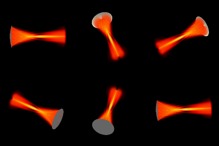
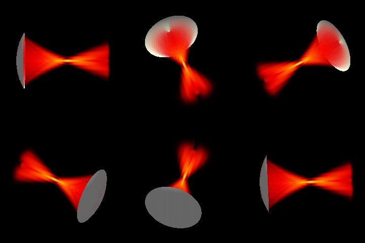
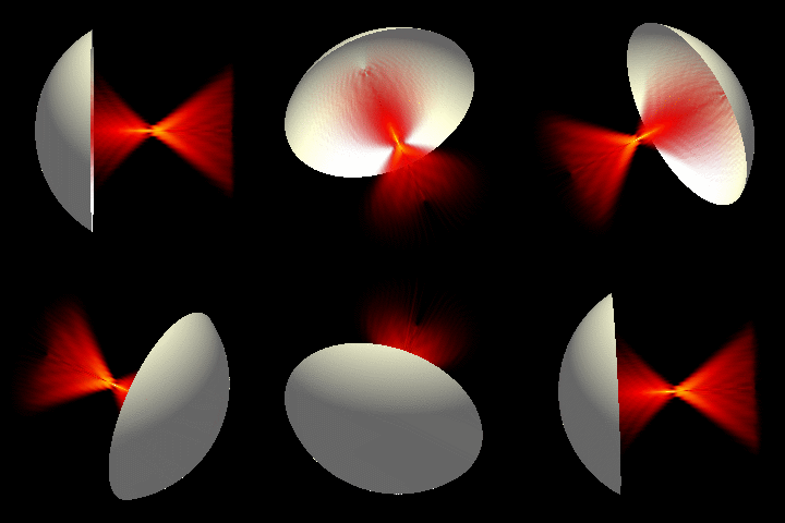
A concave spherical radiator concentrates acoustic energy near its geometric focus. Diffraction gives the focal region a finite width and can shift the pressure maximum toward the transducer relative to that geometric focus.
The F-number is the focal distance divided by the aperture diameter:
\[F_\#=\frac{F}{D},\qquad D=2a.\]Here, \(F\) is the radius of curvature (the geometric focal distance), \(D\) the aperture diameter and \(a\) its radius. At a fixed wavelength, a smaller F-number generally gives a narrower focal main lobe. Gain, focal shift and side lobes also depend on wavelength and aperture illumination.
Three-dimensional field views
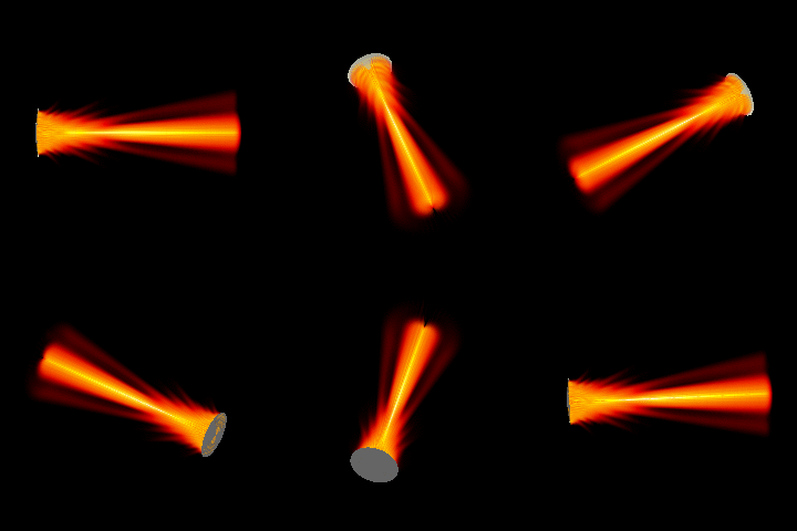
Focused source at \(F_\#=5\)

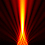
Focused source at \(F_\#=3\)

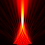
Focused source at \(F_\#=2\)

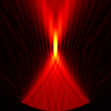
Focused source at \(F_\#=1.25\)

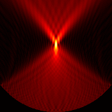
An on-axis approximation
For a uniformly driven spherical aperture, a paraxial, linear, lossless approximation gives useful scaling relations. Define the diffraction length \(L_d\), focusing parameter \(G\) and Fresnel number \(N_F\) by
\[L_d=\frac{ka^2}{2},\qquad G=\frac{L_d}{F},\qquad N_F=\frac{a^2}{\lambda F}=\frac{G}{\pi}.\]With \(\tilde z=z/F\) and reference plane-wave pressure amplitude \(p_{\mathrm{ref}}=\rho_0c_0|v_0|\), the on-axis pressure amplitude is approximately
\[\frac{|\hat p(0,z)|}{p_{\mathrm{ref}}}\simeq \left|\frac{2}{1-\tilde z}\sin\left(\frac{G(1-\tilde z)}{2\tilde z}\right)\right|.\]The apparent singularity at \(z=F\) is removable: the limit is \(G\). This is the gain at the geometric focus under the approximation, rather than necessarily the largest pressure anywhere on the axis. The reference amplitude is not an assertion that the pressure is uniform over the curved transducer face. Strong focusing, nonuniform excitation, absorption and nonlinear propagation require a more complete model.